vif.cca 筛选环境变量:VIF是非常有用的指示符,表明数据集中存在多重共线性。 它不能很好地指示应从模型中删除哪个预测变量。
原文地址:
Variance inflation factors and ordination model selection
Variance inflation factors (VIF) give a measure of the extent of multicollinearity in the predictors of a regression. If the VIF of a predictor is high, it indicates that that predictor is highly correlated with other predictors, it contains little or no unique information, and there is redundancy in the set of predictors.
We don’t really want to have redundant predictors in a constrained ordination: they make the analysis more difficult to interpret, and the more predictors we have, the less constrained the ordination is, the more it resembles an unconstrained ordination.
Model selection in ordinations is tricky. Techniques such as forward selection can guide the choice of predictors to include, but also bias the results (see Juggins 2013).
Recently I have seen a paper and reviewed a manuscript using VIF to determine which predictor to drop from a constrained ordination in a backwards selection.
The procedure they were using was
- Generate a constrained ordination with all available predictors.
- Calculate the VIF of each variable.
- If any variable has a VIF over a threshold (typically 20), drop the variable with the highest VIF
- Repeat until all remaining variables have a VIF below the threshold.
I want to show that this is a procedure that can go badly wrong using an example based on the SWAP diatom-pH calibration set.
First I load the data from the rioja package and make two fake pH variables that are highly correlated with the observed pH by adding Gaussian noise to the observed pH.
library(rioja)
data(SWAP)

env<-data.frame(pH=SWAP$pH, fakepH1=rnorm(length(SWAP$pH), SWAP$pH, .2), fakepH2=rnorm(length(SWAP$pH), SWAP$pH, .2))
pairs(env)#highly correlated.
mod<-cca(sqrt(SWAP$spec)~., env)
vif.cca(mod)
#      pH  fakepH1  fakepH2
#26.82960 12.63575 14.49851
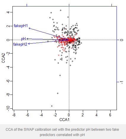
plot(mod)

CCA of the SWAP calibration set with the predictor pH between two fake predictors correlated with pH
The VIF for pH is greater than the threshold 20, and so under the above procedure is dropped. If we fit a new model without pH we find the VIF of the remaining predictors has fallen and all are now below the threshold. An anova shows that both predictors are statistically significant
mod2<-cca(sqrt(SWAP$spec)~.-pH, env)
vif.cca(mod2)
# fakepH1  fakepH2
#6.822985 6.822985

anova(mod2, by="terms")
#Permutation test for cca under reduced model
#Terms added sequentially (first to last)
#
#Model: cca(formula = sqrt(SWAP$spec) ~ (pH + fakepH1 + fakepH2) - pH, data = env)
#          Df   Chisq       F N.Perm Pr(>F)
#fakepH1    1  0.3406 11.0050     99   0.01 **
#fakepH2    1  0.0530  1.7122     99   0.01 **
#Residual 164  5.0754
#---
#Signif. codes:  0 ‘***’ 0.001 ‘**’ 0.01 ‘*’ 0.05 ‘.’ 0.1 ‘ ’ 1
What’s happening is that pH is highly correlated with both fake predictors, whereas the fake predictors are less strongly correlated with each other so have a lower VIF.
Any procedure with a high risk of throwing out the true predictor and instead accepting two fake predictors is not a useful method.
Is my toy example realistic? I would argue it is. One of the studies I saw used the temperature of all the months of a year as predictors for a calibration set. Imagine that June is the true predictor, but June temperature will be highly correlated with May and July temperatures. The procedure risks returning three or four months spaced evenly around the calendar rather than just June.
VIF is a very useful indicator that there is multicollinearity in a data set. It is a poor indicator of which predictor should be dropped from a model.
- 发表于 2020-11-05 14:44
- 阅读 ( 6743 )
- 分类:宏基因组
你可能感兴趣的文章
- 典型相关性分析CCA与冗余分析RDA 13635 浏览
- RDA CCA 分析 17125 浏览
- RDA CCA 分析Hellinger转化问题 13106 浏览
- 排序分析PCA、PCoA、CA、NMDS、RDA、CCA等区别与联系 46425 浏览
相关问题
- vegan包问题请教 1 回答
- vegan包问题请教 0 回答
